Segmentación de clientes
Este trabajo tiene como objetivo realizar un agrupamiento de los clientes de una empresa para entender mejor las distintas características que poseen y establecer estrategias de marketing personalizadas (lo que se conoce como “segmentación de clientes”). El objetivo principal es generar un análisis de clustering y realizar una descripción de las principales características que presentan los clientes que pertenecen a cada clúster.
El dataset que vamos a utilizar es marketing_campaign.csv que se puede econtrarn en el siguiente enlace, además allí se puede encontrar detallada la información de cada uno de los atributos que conforman este dataset.
El trabajo consistirá en tres secciones:
- Preprocesamiento de los datos: extracción, transformación y verificación de la calidad de los datos, selección de las variables de interés, y estandarización de los datos.
- Reducción de dimensionalidad: análisis de PCA sobre los datos, determinando el número de componentes principales óptimo según un criterios previamente establecidos. Realización de un scatterplot (grpafico de puntos) de los primeros componentes principales.
- Clustering: realización de clusters con las técnicas k-means y DBSCAN a partir del resultado del PCA considerando el valor óptimo de k y considerando distintas medidas de validación interna y externa.
Comencemos!
Instalamos e importamos paquetes
# !pip install pandas
# !pip install numpy
# !pip install matplotlib
# !pip install scikit-learn
# !pip install kneed
# !pip install yellow brick
# !pip install plotly
Importamos el dataset
import pandas as pd
import numpy as np

df = pd.read_csv('data/marketing_campaign.csv',delimiter="\t")
Veamos la estructura del dataset
# cantidad de filas y columnas
df.shape
## (2240, 29)# 5 primeras filas
df.head()## ID Year_Birth Education ... Z_CostContact Z_Revenue Response
## 0 5524 1957 Graduation ... 3 11 1
## 1 2174 1954 Graduation ... 3 11 0
## 2 4141 1965 Graduation ... 3 11 0
## 3 6182 1984 Graduation ... 3 11 0
## 4 5324 1981 PhD ... 3 11 0
##
## [5 rows x 29 columns]ZONA PREPROCESADO
1. Exploramos los tipos de datos.
#exploremos los tipos de datos del df
df.dtypes
## ID int64
## Year_Birth int64
## Education object
## Marital_Status object
## Income float64
## Kidhome int64
## Teenhome int64
## Dt_Customer object
## Recency int64
## MntWines int64
## MntFruits int64
## MntMeatProducts int64
## MntFishProducts int64
## MntSweetProducts int64
## MntGoldProds int64
## NumDealsPurchases int64
## NumWebPurchases int64
## NumCatalogPurchases int64
## NumStorePurchases int64
## NumWebVisitsMonth int64
## AcceptedCmp3 int64
## AcceptedCmp4 int64
## AcceptedCmp5 int64
## AcceptedCmp1 int64
## AcceptedCmp2 int64
## Complain int64
## Z_CostContact int64
## Z_Revenue int64
## Response int64
## dtype: object# veamos si hay datos NA
df.isna().sum()## ID 0
## Year_Birth 0
## Education 0
## Marital_Status 0
## Income 24
## Kidhome 0
## Teenhome 0
## Dt_Customer 0
## Recency 0
## MntWines 0
## MntFruits 0
## MntMeatProducts 0
## MntFishProducts 0
## MntSweetProducts 0
## MntGoldProds 0
## NumDealsPurchases 0
## NumWebPurchases 0
## NumCatalogPurchases 0
## NumStorePurchases 0
## NumWebVisitsMonth 0
## AcceptedCmp3 0
## AcceptedCmp4 0
## AcceptedCmp5 0
## AcceptedCmp1 0
## AcceptedCmp2 0
## Complain 0
## Z_CostContact 0
## Z_Revenue 0
## Response 0
## dtype: int64# vamos a eliminar los registros que tienen datos NA en la variable Income
df = df.dropna(subset=['Income'])2. Chequeamos la calidad de los datos (detección de outliers).
# ahora chequeamos la existencia de outliers y los eliminamos
from sklearn.neighbors import LocalOutlierFactor

lof = LocalOutlierFactor()
outlier_scores = lof.fit_predict(df[['Income']])
outlier_scores
## array([1, 1, 1, ..., 1, 1, 1])mask = outlier_scores == -1
df = df.loc[~mask]
df= df.reset_index(drop=True)
sum(outlier_scores == -1)## 243. Limpiamos y ordenamos datos
Vamos a calcular los años de pertenencia a la empresa para cada cliente, la edad actual de cada cliente e intentar agrupar aquellos clientes con hijos tanto niños como adolescentes en una sola variable.
# primero pasamos la variable a tipo fecha
df['Dt_Customer'] = pd.to_datetime(df['Dt_Customer'], format='%d-%m-%Y')

# importamos libreria para operar fechas
from datetime import datetime

# Obtener la fecha actual
fecha_actual = datetime.now()

# Calcular la diferencia en años entre Dt_Customer y la fecha actual
df['años_de_cliente'] = ((fecha_actual - df['Dt_Customer']).dt.total_seconds() / (365.25 * 24 * 3600)).astype(int)
# calculemos la edad de cada cliente
df['Edad'] = 2023 - df['Year_Birth']# agrupamos la variable de niños
df['kids'] = df['Kidhome']+df['Teenhome']4. Seleccionamos variables de interés
Si bien hay muchas variables de tipo numérica, por la descripción del dataset en la web de kaggle, sabemos que algunas son dicotómicas o booleanas. Vamos a armar un nuevo df pero sólo con las variables numéricas.
col_bool = ['Complain', 'AcceptedCmp1', 'AcceptedCmp2', 'AcceptedCmp3', 'AcceptedCmp4', 'AcceptedCmp5', 'Response', 'Kidhome', 'Teenhome']

col_numericas = df.select_dtypes(include=['int64','float64']).drop(columns = col_bool).columns.tolist()

print(col_numericas)
## ['ID', 'Year_Birth', 'Income', 'Recency', 'MntWines', 'MntFruits', 'MntMeatProducts', 'MntFishProducts', 'MntSweetProducts', 'MntGoldProds', 'NumDealsPurchases', 'NumWebPurchases', 'NumCatalogPurchases', 'NumStorePurchases', 'NumWebVisitsMonth', 'Z_CostContact', 'Z_Revenue', 'Edad', 'kids']# nos quedamos con las variables numéricas de interés
df2 = df[col_numericas].drop(columns = ['ID', 'Year_Birth', 'NumWebVisitsMonth', 'Recency', 'Z_CostContact', 'Z_Revenue'])
# chequeo
df2.dtypes## Income float64
## MntWines int64
## MntFruits int64
## MntMeatProducts int64
## MntFishProducts int64
## MntSweetProducts int64
## MntGoldProds int64
## NumDealsPurchases int64
## NumWebPurchases int64
## NumCatalogPurchases int64
## NumStorePurchases int64
## Edad int64
## kids int64
## dtype: object5. Estandarizamos el dataset
Por último, estandarizamos el df con variables numéricas.
# al estandarizar, voy a crear una matriz, para volver a tener un df necesito guardar los nombres de las columnas
cols = df2.columns

# importo librerias
from sklearn.preprocessing import StandardScaler

# creo el estandarizador "vacío"
scaler = StandardScaler()

# fiteo y estandarizo
df2_scaled = scaler.fit_transform(df2)

# paso a df la matriz
df2 = pd.DataFrame(df2_scaled, columns = cols)

# chequeo
df2.describe()
## Income MntWines ... Edad kids
## count 2.192000e+03 2.192000e+03 ... 2.192000e+03 2.192000e+03
## mean 1.247988e-16 -9.076276e-17 ... -1.673438e-16 6.807207e-17
## std 1.000228e+00 1.000228e+00 ... 1.000228e+00 1.000228e+00
## min -2.331354e+00 -9.069508e-01 ... -2.269460e+00 -1.275344e+00
## 25% -7.962301e-01 -8.356721e-01 ... -6.849356e-01 -1.275344e+00
## 50% -1.318419e-02 -3.797857e-01 ... -1.011634e-01 6.160196e-02
## 75% 8.142272e-01 5.928711e-01 ... 8.161931e-01 6.160196e-02
## max 2.159473e+00 3.527176e+00 ... 6.320332e+00 2.735493e+00
##
## [8 rows x 13 columns]ZONA REDUCCIÓN DE LA DIMENSIONALIDAD
1. Llevamos a cabo un PCA con las variables númericas ya estandarizadas del dataset.
from sklearn.decomposition import PCA

pca = PCA()
df_pca = pca.fit_transform(df2)
2. Determinamos el número de componentes principales que serán tenidos en cuenta para los siguientes análisis
import matplotlib.pyplot as plt

def plot_variance(pca, width=8, dpi=100):
    # Create figure
    fig, axs = plt.subplots(1, 2)
    n = pca.n_components_
    grid = np.arange(1, n + 1)
    # Explained variance
    evr = pca.explained_variance_ratio_
    axs[0].bar(grid, evr)
    axs[0].set(
        xlabel="Componente", title="% Varianza Explicada", ylim=(0.0, 1.0)
    )
    # Cumulative Variance
    cv = np.cumsum(evr)
    axs[1].plot(np.r_[0, grid], np.r_[0, cv], "o-")
    axs[1].set(
        xlabel="Componente", title="% Varianza Acumulada", ylim=(0.0, 1.0)
    )
    # Set up figure
    fig.set(figwidth=8, dpi=100)
    return axs

plot_variance(pca)
## array([<Axes: title={'center': '% Varianza Explicada'}, xlabel='Componente'>,
## <Axes: title={'center': '% Varianza Acumulada'}, xlabel='Componente'>],
## dtype=object)pca.explained_variance_ratio_## array([0.45837944, 0.13064097, 0.07715654, 0.06335221, 0.05327535,
## 0.03882232, 0.03309102, 0.03204474, 0.03138168, 0.02946957,
## 0.02130461, 0.01830032, 0.01278122])educacion = df['Education']
valores_unicos_educacion = df['Education'].unique()
print(valores_unicos_educacion)## ['Graduation' 'PhD' 'Master' 'Basic' '2n Cycle']3. Graficamos la distribución de los clientes (observaciones) en los dos primeros componentes principales
educacion = df['Education']

principalDf = pd.DataFrame(data = df_pca[:, :2]
             , columns = ['principal component 1', 'principal component 2'])
finalDf = pd.concat([principalDf, educacion], axis = 1)


#Graficamos la distribución de nuestros puntos en este nuevo espacio

fig = plt.figure(figsize = (8,8))
ax = fig.add_subplot(1,1,1)
ax.set_xlabel('Principal Component 1', fontsize = 15)
ax.set_ylabel('Principal Component 2', fontsize = 15)
ax.set_title('PCA - segmentacion clientes', fontsize = 20)
targets = ['Graduation', 'PhD', 'Master', 'Basic', '2n Cycle']
colors = ['r', 'g', 'b', 'orange', 'yellow']
for target, color in zip(targets,colors):
    indicesToKeep = finalDf['Education'] == target
    ax.scatter(finalDf.loc[indicesToKeep, 'principal component 1']
               , finalDf.loc[indicesToKeep, 'principal component 2']
               , c = color
               , s = 50)
ax.legend(targets)
ax.grid()
plt.show()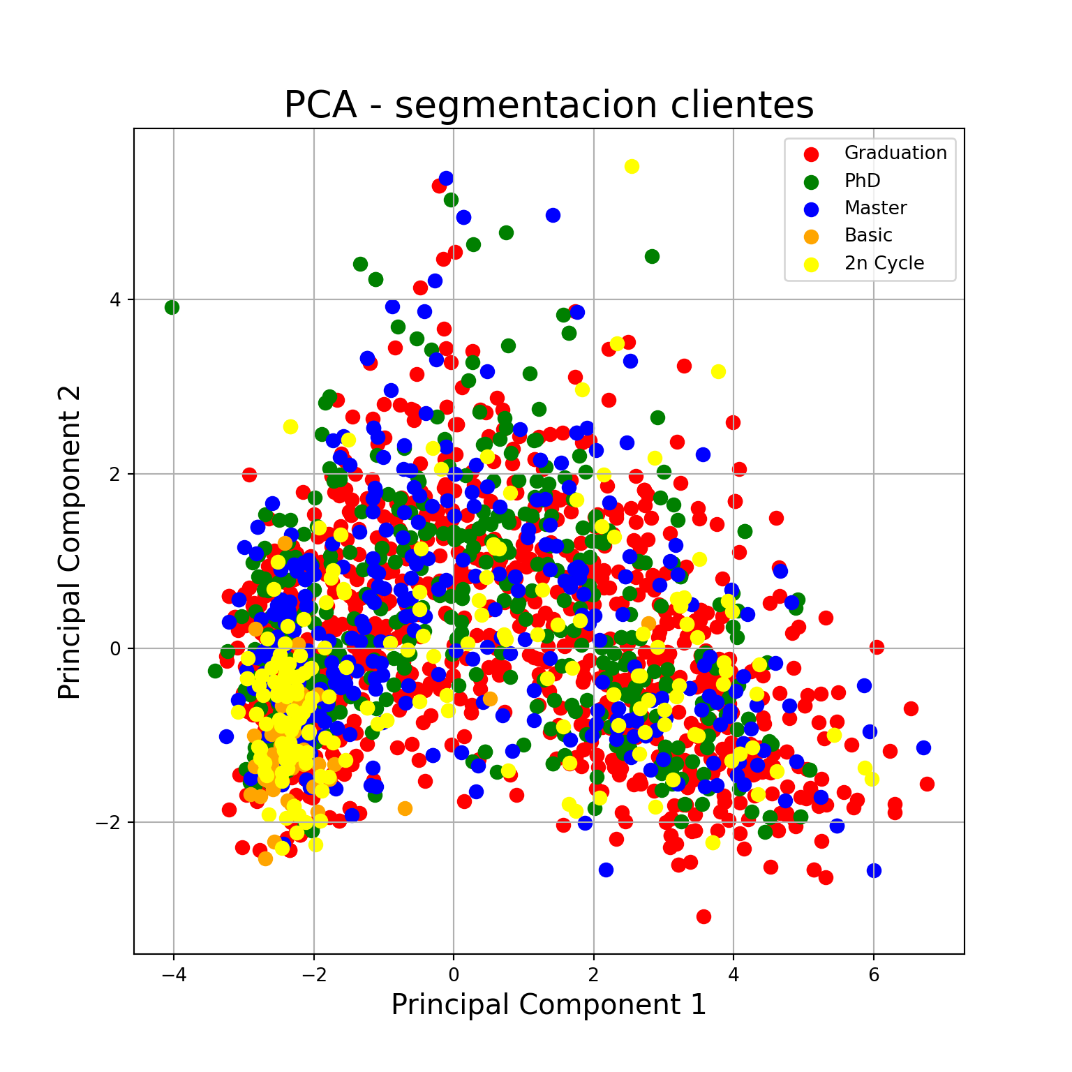
4. Evaluamos cuáles son las variables originales más importantes para los dos primeros componentes
# Convertimos el pca en un dataframe
component_names = [f"PC{i+1}" for i in range(df_pca.shape[1])]
df_pca = pd.DataFrame(df_pca, columns=component_names)

# Chequeamos loadings
loadings = pd.DataFrame(
    pca.components_.T,
    columns=component_names,
    index=df2.columns,
)
loadings
## PC1 PC2 PC3 ... PC11 PC12 PC13
## Income 0.353865 0.080804 0.193249 ... 0.140758 -0.035343 -0.786790
## MntWines 0.316894 0.195387 0.161487 ... -0.368794 0.661305 0.209364
## MntFruits 0.293412 -0.148163 -0.181059 ... -0.163786 0.037281 0.013557
## MntMeatProducts 0.341339 -0.137226 0.047092 ... 0.739464 0.016947 0.320501
## MntFishProducts 0.303241 -0.156104 -0.148121 ... -0.154440 0.175747 0.014417
## MntSweetProducts 0.293481 -0.130538 -0.184517 ... -0.051611 0.099554 0.037425
## MntGoldProds 0.242791 0.120712 -0.266284 ... 0.099767 0.081995 0.009164
## NumDealsPurchases -0.046890 0.618811 -0.377657 ... 0.047324 0.086942 -0.236296
## NumWebPurchases 0.240630 0.410637 -0.132109 ... 0.125325 -0.191648 0.061344
## NumCatalogPurchases 0.348735 0.017284 0.093837 ... -0.455322 -0.653011 0.125240
## NumStorePurchases 0.308511 0.198420 0.004046 ... 0.078168 -0.185551 0.253486
## Edad 0.058169 0.299576 0.775207 ... 0.048473 0.047653 0.056767
## kids -0.233327 0.421386 -0.069551 ... -0.018766 -0.069408 0.299615
##
## [13 rows x 13 columns]ZONA CLUSTERING
1. Antes de comenzar la clusterización, vamos a calcular cuán probable es encontrar clusters en el dataset que venimos trabajando, para esto utilizamos el estadístico de Hopkins.
from numpy.random import uniform
from random import sample
from sklearn.neighbors import NearestNeighbors

# function to compute hopkins's statistic for the dataframe X
def hopkins_statistic(X):

    X=X.values  #convert dataframe to a numpy array
    sample_size = int(X.shape[0]*0.05) #0.05 (5%) based on paper by Lawson and Jures

    #a uniform random sample in the original data space
    X_uniform_random_sample = uniform(X.min(axis=0), X.max(axis=0) ,(sample_size , X.shape[1]))

    #a random sample of size sample_size from the original data X
    random_indices=sample(range(0, X.shape[0], 1), sample_size)
    X_sample = X[random_indices]

    #initialise unsupervised learner for implementing neighbor searches
    neigh = NearestNeighbors(n_neighbors=2)
    nbrs=neigh.fit(X)

    #u_distances = nearest neighbour distances from uniform random sample
    u_distances , u_indices = nbrs.kneighbors(X_uniform_random_sample , n_neighbors=2)
    u_distances = u_distances[: , 0] #distance to the first (nearest) neighbour

    #w_distances = nearest neighbour distances from a sample of points from original data X
    w_distances , w_indices = nbrs.kneighbors(X_sample , n_neighbors=2)
    #distance to the second nearest neighbour (as the first neighbour will be the point itself, with distance = 0)
    w_distances = w_distances[: , 1]

    u_sum = np.sum(u_distances)
    w_sum = np.sum(w_distances)

    #compute and return hopkins' statistic
    H = u_sum/ (u_sum + w_sum)
    return H
Calculamos el valor del estadístico de Hopkins, mientras más cercano a 1 sea, mayor será la probabilidad de encontrar clusters definidos.
# chequeamos el valor del estadístico de Hopkins, cuanto más cercano a 1 mayor probabilidad de encontrar clusters definidos
H=hopkins_statistic(df2)
print(H)
## 0.84684295724137732. Realizaremos un análisis de k-means a partir de la reducción de dimensionalidad realizada en el punto anterior. Para ésto necesitamos determinar el k-óptimo, una forma es con la regla del codo (elbow method).
from sklearn.cluster import KMeans, DBSCAN

kmeans_kwargs = {
    "init": "random",
    "n_init": 10,
    "max_iter": 300,
    "random_state": 42,
}

# SSE: Sum of Square Error
sse = []
for k in range(1, 11):
    kmeans = KMeans(n_clusters=k, **kmeans_kwargs)
    kmeans.fit(df_pca)
    sse.append(kmeans.inertia_)
KMeans(init='random', n_clusters=10, n_init=10, random_state=42)In a Jupyter environment, please rerun this cell to show the HTML representation or trust the notebook.
On GitHub, the HTML representation is unable to render, please try loading this page with nbviewer.org.
KMeans(init='random', n_clusters=10, n_init=10, random_state=42)
fig = plt.figure(figsize = (8,8))
ax = fig.add_subplot(1,1,1)
ax.set_xlabel('Número de Clusters', fontsize = 15)
ax.set_ylabel('SSE', fontsize = 15)
ax.set_title('Número de k-óptimo', fontsize = 20)
ax.set_xticks(range(1, len(sse) + 1))
ax.plot(range(1, len(sse)+1), sse, marker = 'o')
ax.grid()
plt.show()
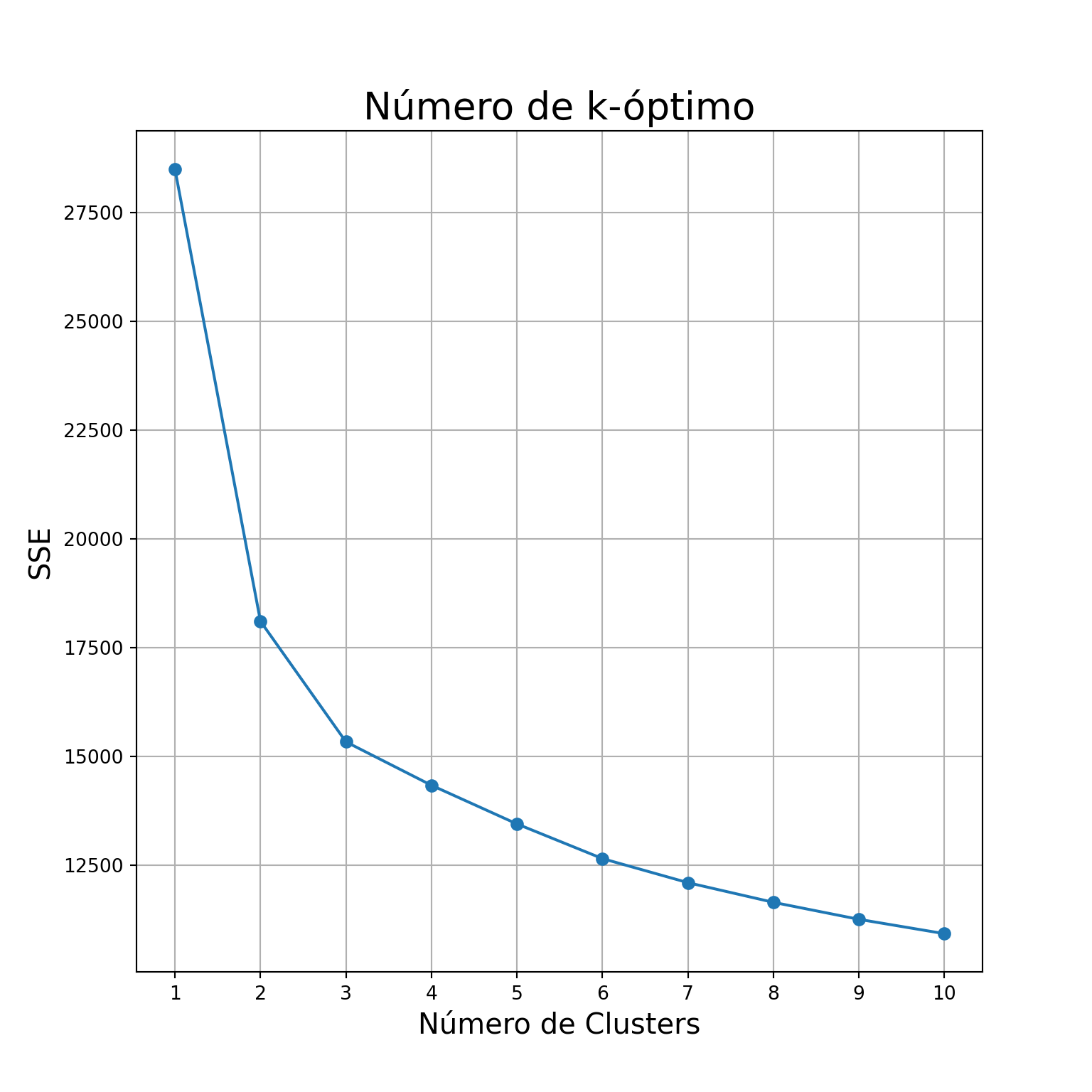
Si ejecutamos el método del elbow, a simple vista pareciera que el número óptimo de clústers está en k = 3, pero podemos confirmarlo con la siguiente función:
from kneed import KneeLocator

kl = KneeLocator(
    range(1, 11), sse, curve="convex", direction="decreasing"
)

kl.elbow
## 3Sabiendo el número de k óptimos, generamos el kmeans:
kmeans = KMeans(
    init="random",
    n_clusters=3,
    n_init=10,
    max_iter=300,
    random_state=42
)

kmeans.fit(df_pca)
KMeans(init='random', n_clusters=3, n_init=10, random_state=42)In a Jupyter environment, please rerun this cell to show the HTML representation or trust the notebook.
On GitHub, the HTML representation is unable to render, please try loading this page with nbviewer.org.
KMeans(init='random', n_clusters=3, n_init=10, random_state=42)
Creamos un df donde guardaremos los valores de clusters obtenidos y graficamos los resultados
# creamos el df
df_pca_results = df_pca

df_pca_results['kmeans'] = kmeans.labels_
# graficamos
fig = plt.figure(figsize = (8,8))
ax = fig.add_subplot(1,1,1)
ax.set_xlabel('Principal Component 1', fontsize = 15)
ax.set_ylabel('Principal Component 2', fontsize = 15)
ax.set_title('PCA + K-means Segmentación de clientes', fontsize = 20)
targets = [0, 1, 2]
colors = ['r', 'g', 'b']
for target, color in zip(targets,colors):
indicesToKeep = df_pca_results['kmeans'] == target
ax.scatter(df_pca_results.loc[indicesToKeep, 'PC1']
, df_pca_results.loc[indicesToKeep, 'PC2']
, c = color
, s = 50)
ax.legend(targets)
ax.grid()
plt.show()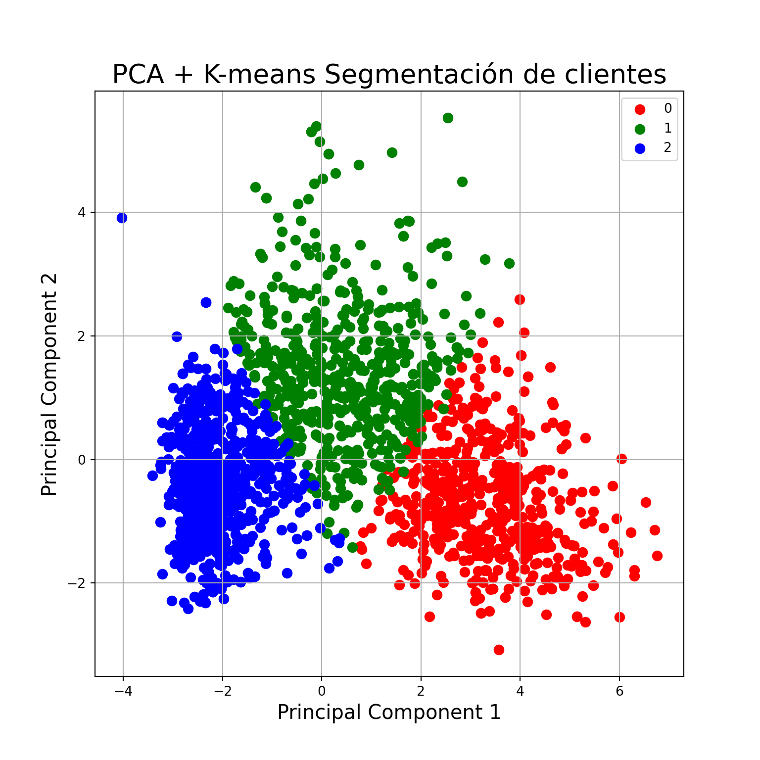
3. Implementaremos un segúndo método de clustering sobre los datos, elegimos el algoritmo DBSCAN:
k = 2
# Nos quedamos con los 3 primero PC
data_nn = df_pca.loc[:,['PC1', 'PC2', 'PC3']]


# Calculamos los vecinos más cercanos
nearest_neighbors = NearestNeighbors(n_neighbors=k)
neighbors = nearest_neighbors.fit(data_nn)
distances, indices = neighbors.kneighbors(data_nn)
distances = np.sort(distances, axis=0)

# Obtenemos las distancias
distances = distances[:,1]

i = np.arange(len(distances))

import seaborn as sns

sns.lineplot(
    x = i,
    y = distances
)
plt.axhline(y = 0.4, color = 'r', linestyle = '--')
plt.xlabel("Observaciones", fontsize = 15)
plt.ylabel("Distancia", fontsize = 15)
plt.grid()
plt.show()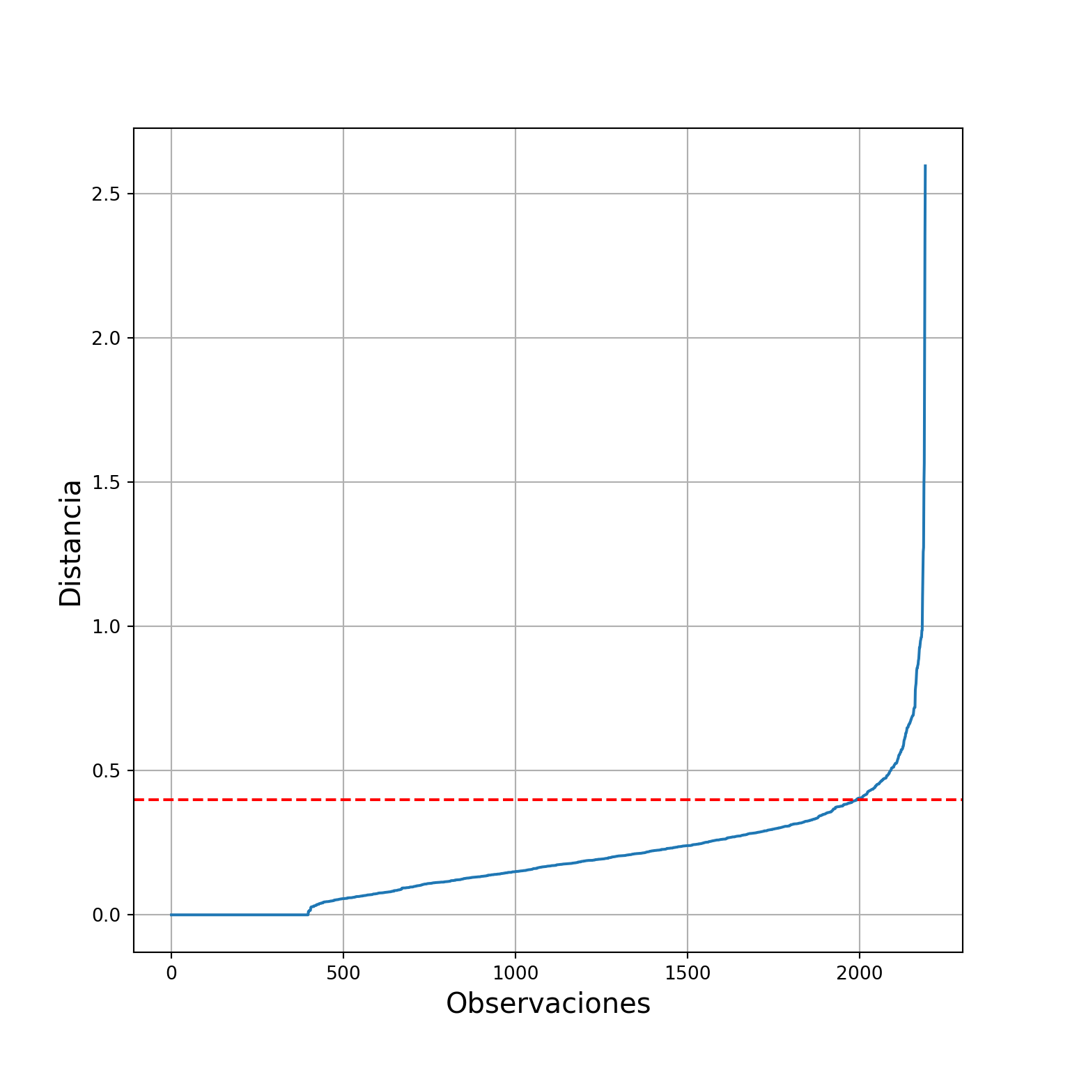
#Realizamos el clustering
dbscan_clusters = DBSCAN(eps = 0.4, min_samples = 4).fit(data_nn)
# guardamos los resultados
df_pca_results['dbscan_pca'] = pd.Series(dbscan_clusters.labels_)#Veamos que tal le fue
fig = plt.figure(figsize = (8,8))
ax = fig.add_subplot(1,1,1)
ax.set_xlabel('Principal Component 1', fontsize = 15)
ax.set_ylabel('Principal Component 2', fontsize = 15)
ax.set_title('PCA + DBSCAN Segmentación de clientes', fontsize = 20)
targets = [-1, 0, 1]
colors = ['gray', 'r', 'g']
for target, color in zip(targets,colors):
indicesToKeep = df_pca_results['dbscan_pca'] == target
ax.scatter(df_pca_results.loc[indicesToKeep, 'PC1']
, df_pca_results.loc[indicesToKeep, 'PC2']
, c = color
, s = 50)
ax.legend(targets)
ax.grid()
plt.show()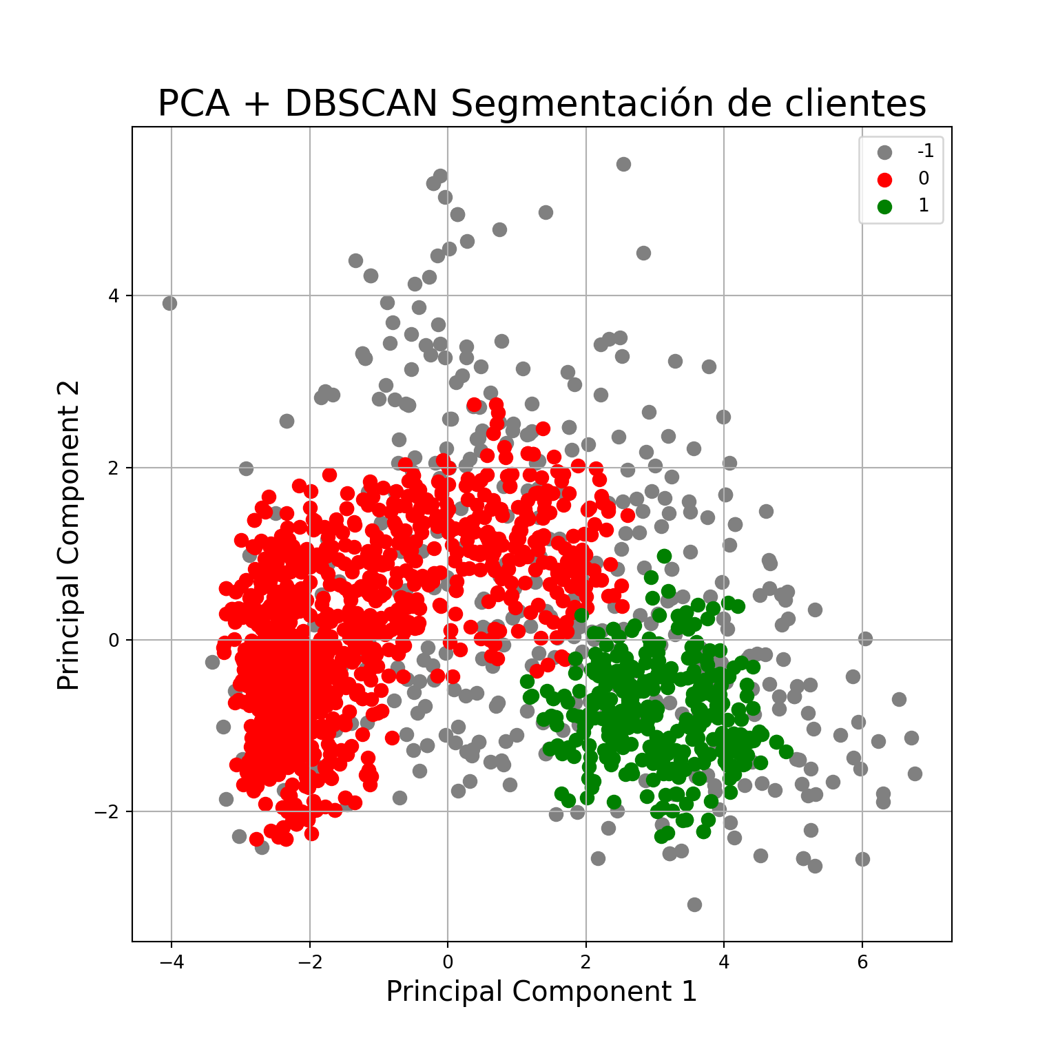
4. Realizaremos una validación interna del clustering k-means con el k-seleccionado. Compararemos el resultado con otro clustering con un k distinto
# generamos un kmeans con 5 clusters
kmeans_5 = KMeans(
    init="random",
    n_clusters=5,
    n_init=10,
    max_iter=300,
    random_state=42
)

kmeans_5.fit(df_pca)
KMeans(init='random', n_clusters=5, n_init=10, random_state=42)In a Jupyter environment, please rerun this cell to show the HTML representation or trust the notebook.
On GitHub, the HTML representation is unable to render, please try loading this page with nbviewer.org.
KMeans(init='random', n_clusters=5, n_init=10, random_state=42)
df_pca_results['kmeans_5'] = kmeans_5.labels_# comapramos ambos kmeans
from sklearn.metrics import davies_bouldin_score, silhouette_score
print("davies_bouldin para k = 3: ", davies_bouldin_score(df_pca, df_pca_results['kmeans']))## davies_bouldin para k = 3: 2.3402509584444826print("davies_bouldin para k = 5: ", davies_bouldin_score(df2, df_pca_results['kmeans_5']))
# davies_bouldin cuanto menor, mejor## davies_bouldin para k = 5: 5.664165728007428print("silhouette_score para k = 3: ", silhouette_score(df_pca, df_pca_results['kmeans']))## silhouette_score para k = 3: 0.29289601103113794print("silhouette_score para k = 5: ", silhouette_score(df2, df_pca_results['kmeans_5']))
#silhouette_score cuanto mayor, mejor## silhouette_score para k = 5: 0.23902485138025292from yellowbrick.cluster import silhouette_visualizer
#Kmeans con k=3 (el que elegimos)
silhouette_visualizer(KMeans(3, n_init=10, random_state=42), df_pca, colors='yellowbrick')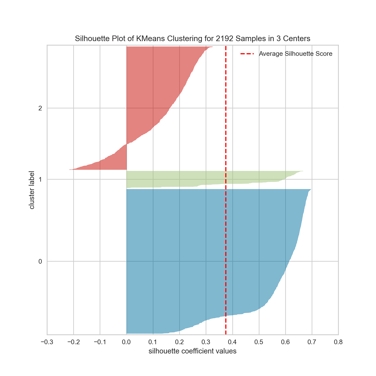
SilhouetteVisualizer(ax=<Axes: >, colors='yellowbrick',
                     estimator=KMeans(n_clusters=3, n_init=10, random_state=42))
In a Jupyter environment, please rerun this cell to show the HTML representation or trust the notebook. On GitHub, the HTML representation is unable to render, please try loading this page with nbviewer.org.
SilhouetteVisualizer(ax=<Axes: >, colors='yellowbrick',
estimator=KMeans(n_clusters=3, n_init=10, random_state=42))KMeans(n_clusters=3, n_init=10, random_state=42)
KMeans(n_clusters=3, n_init=10, random_state=42)
#Kmeans con k=5
silhouette_visualizer(KMeans(5, n_init=10, random_state=42), df_pca, colors='yellowbrick')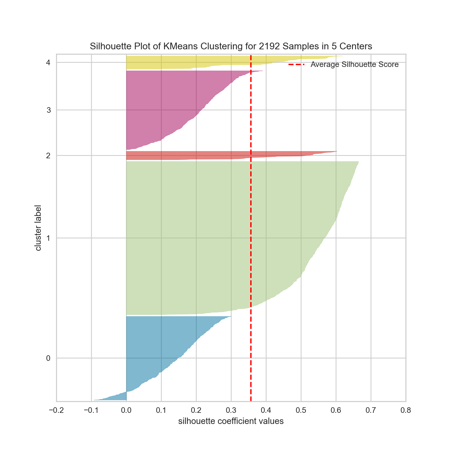
SilhouetteVisualizer(ax=<Axes: >, colors='yellowbrick',
                     estimator=KMeans(n_clusters=5, n_init=10, random_state=42))
In a Jupyter environment, please rerun this cell to show the HTML representation or trust the notebook. On GitHub, the HTML representation is unable to render, please try loading this page with nbviewer.org.
SilhouetteVisualizer(ax=<Axes: >, colors='yellowbrick',
estimator=KMeans(n_clusters=5, n_init=10, random_state=42))KMeans(n_clusters=5, n_init=10, random_state=42)
KMeans(n_clusters=5, n_init=10, random_state=42)
5. Realizaremos una validación externa tomando como “información externa” alguna de las variables categóricas del dataset: Education o Marital_Status y veremos si están relacionadas con los grupos que se establecen.
valores_unicos_educacion = df['Education'].unique()
valores_unicos_marital = df['Marital_Status'].unique()

print(valores_unicos_educacion)
## ['Graduation' 'PhD' 'Master' 'Basic' '2n Cycle']print(valores_unicos_marital)## ['Single' 'Together' 'Married' 'Divorced' 'Widow' 'Alone' 'Absurd' 'YOLO']#agrupamos en 3 niveles los niveles educativos
mapping = {
'Basic': 1,
'Graduation': 2,
'2n Cycle': 2,
'PhD': 3,
'Master': 3
}
# Aplicar el mapeo a la columna 'education'
df['Education'] = df['Education'].map(mapping)#Para kmeans
from sklearn.metrics.cluster import adjusted_rand_score
labels_true = df['Education']
labels_pred = df_pca_results['kmeans']
adjusted_rand_score(labels_true, labels_pred)## 0.0021053589326443267INTERPRETACION
Intentaremos caracterizar a los clientes en base a los clústers que construimos.
df["cluster"] = kmeans.labels_#Covarianza
c = df2.cov()
# Heatmap
sns.heatmap(c)
plt.show()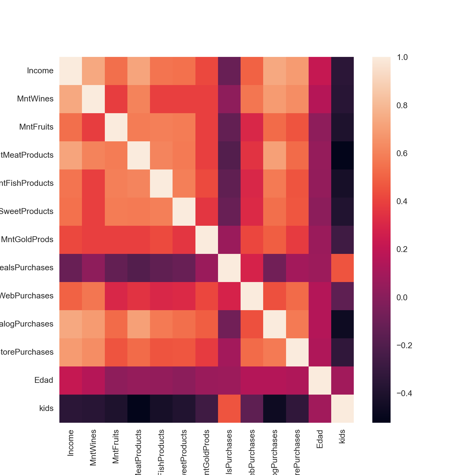
c## Income MntWines ... Edad kids
## Income 1.000456 0.733696 ... 0.216033 -0.348983
## MntWines 0.733696 1.000456 ... 0.161637 -0.355902
## MntFruits 0.541042 0.385926 ... 0.019702 -0.399058
## MntMeatProducts 0.725176 0.604192 ... 0.047739 -0.522433
## MntFishProducts 0.554618 0.392440 ... 0.039997 -0.430983
## MntSweetProducts 0.547867 0.391039 ... 0.017292 -0.388631
## MntGoldProds 0.418044 0.390342 ... 0.065993 -0.271501
## NumDealsPurchases -0.113048 0.022664 ... 0.069293 0.459104
## NumWebPurchases 0.496582 0.563954 ... 0.150189 -0.148759
## NumCatalogPurchases 0.733903 0.690335 ... 0.149917 -0.463843
## NumStorePurchases 0.685928 0.637602 ... 0.132405 -0.328131
## Edad 0.216033 0.161637 ... 1.000456 0.087452
## kids -0.348983 -0.355902 ... 0.087452 1.000456
##
## [13 rows x 13 columns]df.dtypes## ID int64
## Year_Birth int64
## Education int64
## Marital_Status object
## Income float64
## Kidhome int64
## Teenhome int64
## Dt_Customer datetime64[ns]
## Recency int64
## MntWines int64
## MntFruits int64
## MntMeatProducts int64
## MntFishProducts int64
## MntSweetProducts int64
## MntGoldProds int64
## NumDealsPurchases int64
## NumWebPurchases int64
## NumCatalogPurchases int64
## NumStorePurchases int64
## NumWebVisitsMonth int64
## AcceptedCmp3 int64
## AcceptedCmp4 int64
## AcceptedCmp5 int64
## AcceptedCmp1 int64
## AcceptedCmp2 int64
## Complain int64
## Z_CostContact int64
## Z_Revenue int64
## Response int64
## años_de_cliente int32
## Edad int64
## kids int64
## cluster int32
## dtype: objectVeamos cuáles variables fueron más influyentes en el PCA.
# pasamos a positivo todos los valores
df_variables_imp = loadings.abs()

# calculamos el promedio del valor de loading para las 3 primeras PC
df_variables_imp['mean'] = df_variables_imp[['PC1', 'PC2', 'PC3']].mean(axis=1)

# ordenamos
df_variables_imp = df_variables_imp[['PC1', 'PC2', 'PC3','mean']].sort_values(by='mean', ascending=False)

# inspeccionamos
df_variables_imp
## PC1 PC2 PC3 mean
## Edad 0.058169 0.299576 0.775207 0.377651
## NumDealsPurchases 0.046890 0.618811 0.377657 0.347786
## NumWebPurchases 0.240630 0.410637 0.132109 0.261125
## kids 0.233327 0.421386 0.069551 0.241422
## MntWines 0.316894 0.195387 0.161487 0.224589
## MntGoldProds 0.242791 0.120712 0.266284 0.209929
## Income 0.353865 0.080804 0.193249 0.209306
## MntFruits 0.293412 0.148163 0.181059 0.207544
## MntSweetProducts 0.293481 0.130538 0.184517 0.202845
## MntFishProducts 0.303241 0.156104 0.148121 0.202489
## MntMeatProducts 0.341339 0.137226 0.047092 0.175219
## NumStorePurchases 0.308511 0.198420 0.004046 0.170326
## NumCatalogPurchases 0.348735 0.017284 0.093837 0.153285Pareciera que las variables que más influyeron en el cálculo de los PC son Edad, años_de_cliente y NumDealsPurchases
#graficamos

import plotly.express as px

fig = px.scatter_3d(df, x='Edad', y='Income', z='NumDealsPurchases', color='cluster')


fig.update_layout(
    title='Gráfico PC1, PC2 y PC3 - KMEANS CLUSTERING',
    xaxis=dict(title='Edad'),
    yaxis=dict(title='Income'),
    scene=dict(zaxis=dict(title='NumDealsPurchases')),
    coloraxis_colorbar=dict(title='Clusters'),
    width=800,
    height=800
)
Finalmente, según los promedios calculados de los loadings para cada PC, las variables que más influyen en la segmentación de clientes son la Edad, los años_de_cliente y NumDealsPurchases. Sin embargo, las variables años_de_cliente y kids, al tener sólo 3 valores únicos, actúan casi como variables de tipo categóricas, por lo que se decidió graficar la variable Income logrando una mejor aglomeración, es decir más homogénea de los clientes.